Archivo:Mplwp universe scale evolution.svg

Tamaño de esta previsualización PNG del archivo SVG: 600 × 450 píxeles. Otras resoluciones: 320 × 240 píxeles · 640 × 480 píxeles · 1024 × 768 píxeles · 1280 × 960 píxeles · 2560 × 1920 píxeles.
Ver la imagen en su resolución original ((Imagen SVG, nominalmente 600 × 450 pixels, tamaño de archivo: 57 kB))
Resumen
| Descripción |
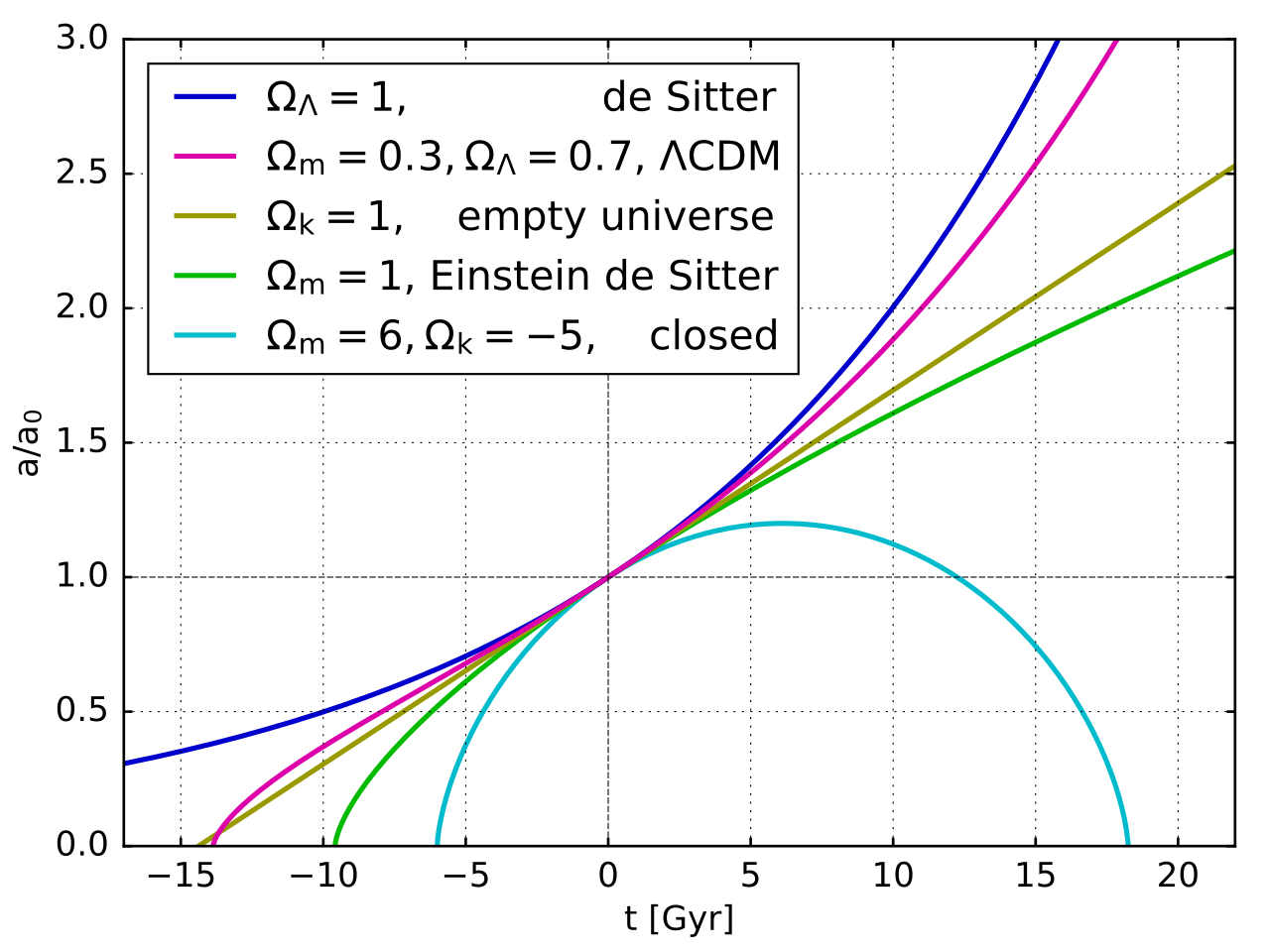
English: Plot of the evolution of the size of the universe (scale parameter a) over time (in billion years, Gyr). Different models are shown, which are all solutions to the Friedmann equations with different parameters. The evolution is governed by the equation
Here is the radiation density, the matter density, the curvature parameter and the dark energy, all normalized such that represents the fact that today's expansion rate is .
|
| Fecha | |
| Fuente | Trabajo propio |
| Autor | Geek3 |
| SVG desarrollo | El código fuente de esta imagen SVG es válido. |
| Código fuente | Python code#!/usr/bin/python
# -*- coding: utf8 -*-
import matplotlib.pyplot as plt
import matplotlib as mpl
import numpy as np
from math import *
code_website = 'http://commons.wikimedia.org/wiki/User:Geek3/mplwp'
try:
import mplwp
except ImportError, er:
print 'ImportError:', er
print 'You need to download mplwp.py from', code_website
exit(1)
name = 'mplwp_universe_scale_evolution.svg'
fig = mplwp.fig_standard(mpl)
fig.set_size_inches(600 / 72.0, 450 / 72.0)
mplwp.set_bordersize(fig, 58.5, 16.5, 16.5, 44.5)
xlim = -17, 22; fig.gca().set_xlim(xlim)
ylim = 0, 3; fig.gca().set_ylim(ylim)
mplwp.mark_axeszero(fig.gca(), y0=1)
import scipy.optimize as op
from scipy.integrate import odeint
tH = 978. / 68. # Hubble time in Gyr
def Hubble(a, matter, rad, k, darkE):
# the Friedman equation gives the relative expansion rate
a = a[0]
if a <= 0: return 0.
r = rad / a**4 + matter / a**3 + k / a**2 + darkE
if r < 0: return 0.
return sqrt(r) / tH
def scale(t, matter, rad, k, darkE):
return odeint(lambda a, t: a*Hubble(a, matter, rad, k, darkE), 1., [0, t])
def scaled_closed_matteronly(t, m):
# analytic solution for matter m > 1, rad=0, darkE=0
t0 = acos(2./m-1) * 0.5 * m / (m-1)**1.5 - 1. / (m-1)
try: psi = op.brentq(lambda p: (p - sin(p))*m/2./(m-1)**1.5
- t/tH - t0, 0, 2 * pi)
except Exception: psi=0
a = (1.0 - cos(psi)) * m * 0.5 / (m-1.)
return a
# De Sitter http://en.wikipedia.org/wiki/De_Sitter_universe
matter=0; rad=0; k=0; darkE=1
t = np.linspace(xlim[0], xlim[-1], 5001)
a = [scale(tt, matter, rad, k, darkE)[1,0] for tt in t]
plt.plot(t, a, zorder=-2,
label=ur'$\Omega_\Lambda=1$, de Sitter')
# Standard Lambda-CDM https://en.wikipedia.org/wiki/Lambda-CDM_model
matter=0.3; rad=0.; k=0; darkE=0.7
t0 = op.brentq(lambda t: scale(t, matter, rad, k, darkE)[1,0], -20, 0)
t = np.linspace(t0, xlim[-1], 5001)
a = [scale(tt, matter, rad, k, darkE)[1,0] for tt in t]
plt.plot(t, a, zorder=-1,
label=ur'$\Omega_m=0.\!3,\Omega_\Lambda=0.\!7$, $\Lambda$CDM')
# Empty universe
matter=0; rad=0; k=1; darkE=0
t0 = op.brentq(lambda t: scale(t, matter, rad, k, darkE)[1,0], -20, 0)
t = np.linspace(t0, xlim[-1], 5001)
a = [scale(tt, matter, rad, k, darkE)[1,0] for tt in t]
plt.plot(t, a, label=ur'$\Omega_k=1$, empty universe', zorder=-3)
'''
# Open Friedmann
matter=0.5; rad=0.; k=0.5; darkE=0
t0 = op.brentq(lambda t: scale(t, matter, rad, k, darkE)[1,0], -20, 0)
t = np.linspace(t0, xlim[-1], 5001)
a = [scale(tt, matter, rad, k, darkE)[1,0] for tt in t]
plt.plot(t, a, label=ur'$\Omega_m=0.\!5, \Omega_k=0.5$')
'''
# Einstein de Sitter http://en.wikipedia.org/wiki/Einstein–de_Sitter_universe
matter=1.; rad=0.; k=0; darkE=0
t0 = op.brentq(lambda t: scale(t, matter, rad, k, darkE)[1,0], -20, 0)
t = np.linspace(t0, xlim[-1], 5001)
a = [scale(tt, matter, rad, k, darkE)[1,0] for tt in t]
plt.plot(t, a, label=ur'$\Omega_m=1$, Einstein de Sitter', zorder=-4)
'''
# Radiation dominated
matter=0; rad=1.; k=0; darkE=0
t0 = op.brentq(lambda t: scale(t, matter, rad, k, darkE)[1,0], -20, 0)
t = np.linspace(t0, xlim[-1], 5001)
a = [scale(tt, matter, rad, k, darkE)[1,0] for tt in t]
plt.plot(t, a, label=ur'$\Omega_r=1$')
'''
# Closed Friedmann
matter=6; rad=0.; k=-5; darkE=0
t0 = op.brentq(lambda t: scaled_closed_matteronly(t, matter)-1e-9, -20, 0)
t1 = op.brentq(lambda t: scaled_closed_matteronly(t, matter)-1e-9, 0, 20)
t = np.linspace(t0, t1, 5001)
a = [scaled_closed_matteronly(tt, matter) for tt in t]
plt.plot(t, a, label=ur'$\Omega_m=6, \Omega_k=\u22125$, closed', zorder=-5)
plt.xlabel('t [Gyr]')
plt.ylabel(ur'$a/a_0$')
plt.legend(loc='upper left', borderaxespad=0.6, handletextpad=0.5)
plt.savefig(name)
mplwp.postprocess(name)
|


Licencia
Yo, el titular de los derechos de autor de esta obra, la publico en los términos de la siguiente licencia:
Este archivo está disponible bajo la licencia Creative Commons Attribution-Share Alike 4.0 International.
- Eres libre:
- de compartir – de copiar, distribuir y transmitir el trabajo
- de remezclar – de adaptar el trabajo
- Bajo las siguientes condiciones:
- atribución – Debes otorgar el crédito correspondiente, proporcionar un enlace a la licencia e indicar si realizaste algún cambio. Puedes hacerlo de cualquier manera razonable pero no de manera que sugiera que el licenciante te respalda a ti o al uso que hagas del trabajo.
- compartir igual – En caso de mezclar, transformar o modificar este trabajo, deberás distribuir el trabajo resultante bajo la misma licencia o una compatible como el original.
Historial del archivo
Haz clic sobre una fecha y hora para ver el archivo tal como apareció en ese momento.
| Fecha y hora | Miniatura | Dimensiones | Usuario | Comentario | |
|---|---|---|---|---|---|
| actual | 00:12 17 abr 2017 | | 600 × 450 (57 kB) | Geek3 | validator fix |
| 22:33 16 abr 2017 |  | 600 × 450 (57 kB) | Geek3 | {{Information |Description ={{en|1=Plot of the evolution of the size of the universe (scale parameter ''a'') over time (in billion years, Gyr). Different models are shown, which are all solutions to the {{W|Friedmann equations|Friedmann equations}}... |
Usos del archivo
Las siguientes páginas usan este archivo:
Uso global del archivo
Las wikis siguientes utilizan este archivo:
- Uso en ar.wikipedia.org
- Uso en az.wikipedia.org
- Uso en bg.wikipedia.org
- Uso en de.wikipedia.org
- Uso en en.wikipedia.org
- Uso en fa.wikipedia.org
- Uso en fr.wikipedia.org
- Uso en hr.wikipedia.org
- Uso en it.wikipedia.org
- Uso en it.wikiquote.org
- Uso en sr.wikipedia.org
- Uso en ta.wikipedia.org
- Uso en vi.wikipedia.org